Curacy of numerical solutions received by Finite Difference Time Domain (fdtd) method and Godunov's method at the solution of the cable equations is carried out

Вид материала

Содержание

Key words
РЕШЕНИЕ ТЕЛЕГРАФНЫХ УРАВНЕНИЙ МЕТОДОМ КОНЕЧНЫХ РАЗНОСТЕЙ ВО ВРЕМЕННОЙ ОБЛАСТИ ( метод FDTD)
Ключевые слова
2. The comparison of the FDTD method with Godunov’s finite difference scheme

Подобный материал:

PROBLEMELE ENERGETICII REGIONALE № 1 (12) 2010

THE SOLUTION OF THE CABLE EQUATIONS BY MEANS OF FINITE DIFFERENCE TIME DOMAIN METHOD

Patsiuk V., Ribacova G.

Institute of Power Engineering, Academy of Sciences of Moldova

Moldova State University

E-mail: patsiuk@usm.md, gal_rib@mail.ru

Abstract. The analysis and comparison of accuracy of numerical solutions received by Finite Difference Time Domain (FDTD) method and Godunov's method at the solution of the cable equations is carried out. It is demonstrated, that at sudden short circuits and at transition to idling mode in numerical solutions received by means of FDTD method for long lines with the distributed parameters appear strong nonphysical oscillations. It is shown, that the settlement scheme offered by authors on the basis of Godunov's method is deprived these lacks and provides high accuracy for the numerical solutions received at the analysis of dynamic modes in long lines, caused by sudden short circuits and line transitions in an idling mode.

Key words: cable equations, finite difference time domain method, Godunov’s scheme.

OBŢINEREA SOLUŢIILOR ECUAŢIILOR TELEGRAFIŞTILOR CU METODA DIFERENŢELOR FINITE ÎN DOMENIUL DE TIMP (metoda FDT)

Paţiuk V., Rîbacova G.

Institutul de Energetică al AŞM, Universitatea de Stat a Moldovei

Rezumat. S-au analizat şi comparat precizia schemelor de calcul Finite Difference Time Domain (metoda FDTD) şi a schemei numerice de calcul propusă de către Godunov (metoda Godunov) la obţinerea soluţiilor numerice pa ecuaţiilor telegrafiştilor. S-a demonstrat, că în soluţia numerică obţinută în baza metodei FDTT privind procesele dinamice în liniile electrice cu parametri distribuiţi apar oscilaţii puternice, ce nu au provenienţă de origine fizică. Schema modificată de calcul numeric propusă de autori (metoda Godunov) este lipsită de acest dezavantaj şi asigură o precizie mai ridicată la analiza regimurilor de mers în gol şi de scurtcircuit în liniile electrice, care au un caracter aleatoriu de apariţie.

Cuvinte-cheie: ecuaţiile telegrafiştilor, metoda FDTD, schema Godunov.

РЕШЕНИЕ ТЕЛЕГРАФНЫХ УРАВНЕНИЙ МЕТОДОМ КОНЕЧНЫХ РАЗНОСТЕЙ ВО ВРЕМЕННОЙ ОБЛАСТИ ( метод FDTD)

Пацюк В.И., Рыбакова Г

Институт энергетики АНМ, Государственный университет Молдовы

Аннотация. Проведен анализ и сравнение точности численных решений, полученных методом Finite Difference Time Domain (FDTD) и методом Годунова при решении телеграфных уравнений. Показано, что при внезапных коротких замыканиях и при переходе в режим холостого хода в численных решениях полученных с помощью метода FDTD для длинных линий с распределенными параметрами появляются сильные нефизические осцилляции. Показано, что предложенная авторами на основе метода Годунова расчетная схема лишена этих недостатков и обеспечивает высокую точность для численных решений, полученных при анализе динамических режимов в длинных линиях, характеризуемых внезапными короткими замыканиями и переходами линии в режим холостого хода.

Ключевые слова: телеграфные уравнения, метод FDTD, схема Годунова.

Introduction

The (FDTD) method is a computational electrodynamics modeling technique based on non-standard discretization of the Maxwell’s equations over the time and space variables.

The FDTD method belongs to the general class of grid-based differential time-domain numerical modeling methods. The Maxwell’s equations are discretized using central-difference approximations to the space and time partial derivatives. The resulting finite-difference equations are solved in either software or hardware manner so as the computed fields are separated in time by a half of the discretization step. The process of the field computation at the grid cells is repeated over and over again until the desired solution is fully evolved at the required time interval.

The basic FDTD algorithm was proposed firstly in 1966 by Kane Yee [1] (The University of California). However, the descriptor "finite-difference time-domain" and its corresponding "FDTD" acronym were originated by Allen Taflove [2, 3] (Northwestern University, Illinois).

Since about 1990, FDTD techniques have emerged as primary means to computational modeling of many scientific and engineering problems dealing with electromagnetic wave interactions with material structures. Its successful applications range from ultralow-frequency electromagnetic waves in geophysics (involving the ionosphere processes) through microwaves (radar signature technology, antennas and wireless communications devices, including digital devices) to visible light (photonic crystals, nanoplasmonics, solitons and biophotonics). In 2006, an estimated two thousands FDTD-related publications appeared in the science and engineering literature.

Now we are going to consider the application of the FDTD method to the telegraph equations (which can be considered as a particular case of the Maxwell’s equations) and to compare this technique with the Godunov’s finite difference scheme. The last one has been successfully used by authors for numerical solution of wide range of problems modeling the electrical energy transmission in long lines [4].

1. The finite difference scheme of the FDTD method

Let consider the twin-wire line with the length l. The current and the potential wave propagation along the line can be described by telegraph equations

. (1.1)

Here the i(x,t) and u(x,t) are the current and the voltage functions in the line; L and C are the inductance and the capacity distributed along the line; R is the longitudinal active (ohmic) resistance and G is the shunt (transverse) conductance.

Let the electrical circuit has the following initial current and voltage distribution along the line

. (1.2)

Let at the initial time moment t = 0 the circuit is connected to the external voltage source

when

, (1.3)

and its receiving end is closed to the active load by the resistance R_S:

when

. (1.4)

To apply the method, at first on the domain

we generate two grids with integer

and half-integer

nodes. The grid step h over the space variable is calculated as

, and the step  over the time variable is chosen according to the scheme stability condition as

, where

is the velocity of the electromagnetic wave propagation. Thus, we have

;

.

The main idea of the FDTD method is the follows: the current function

is calculated at the integer nodes of the grid

, but the voltage function

is calculated at the half-integer nodes of the grid

. In this case, the derivatives from the equations (1.1) can be approximated by finite differences with second order of accuracy with respect to parameters h and . In this way, we obtain the following finite difference scheme

;

. (1.5)

The equations (1.5) are to be completed by the approximations of the initial and boundary conditions. In order to obtain the second order approximation for the initial condition (1.2) we assume

. (1.6)

The boundary condition at the input of the line (1.3) takes the form

, (1.7)

and the condition (1.4) at the output becomes

. (1.8)

2. The comparison of the FDTD method with Godunov’s finite difference scheme

The Godunov’s finite difference scheme for telegraph equations is elaborated and investigated in details by authors in [4]. Let adduce the main computational formulas of this scheme. The finite difference equations for (1.1) approximation have the following form

;

;

(2.1)

;

.

The approximations for the initial conditions (1.2) take the form

, (2.2)

and for boundary conditions (1.3), (1.4) we obtain

; (2.3)

. (2.4)

The scheme (2.1) – (2.4) possesses the first order of accuracy and is monotonous, i.e. the scheme does not admit the appearance of the nonphysical oscillation when computing the discontinuous solution.

Let compare the accuracy of the solution of the problem (1.1)–(1.4) with the following values of the non-dimensional parameters: L = C = 1; R = G = 0.48; R_S = 3; l = 0.7. We consider the voltage and current equal to zero at t = 0 (

;

) and the sinusoidal voltage at the input point of the line:

. The computations were carried out up to the time moment t = T_max = 4.

The table below contains the results of the comparison of exact analytical solution for current at the output point of the line I_a(t) with the approximate solution I_F(t), obtained by FDTD method and with approximate solution I_G(t), obtained by Godunov’s scheme. There are used the following notations:

and

are the maximal values of the differences between the solutions,

and

are the corresponding mean square deviations. The first column of the table contains the numbers of grid nodes over the space variable.

Table

Accuracy of numerical decisions received by method FDTD and under Godunov's scheme

N
10	0.011108	0.026568	0.013233	0.027565
20	0.002734	0.013365	0.003232	0.013599
40	0.000681	0.006638	0.000800	0.006736
80	0.000170	0.003308	0.000200	0.003357
160	0.000043	0.001651	0.000050	0.001674

The analysis of the given data clearly illustrates the theoretical accuracy of these two methods: the decreasing in two times of the grid step leads to the four times decreasing of the FDTD method error and to the two times decreasing of the Godunov’s scheme error (the second order of accuracy for the FDTD method and the first order – for the Godunov’s scheme). In such a way, for continuous solutions of the problem (1.1)–(1.4) the FDTD method is more exact and, correspondingly, more preferable.

Now let consider the same problem, but with condition that during some period of time at the input of the line the short-circuit occurs, i.e. the input voltage becomes zero in some period of time:

when

and

when

. The time dependences of the voltages and currents at the input of the line (x = 0) for N = 10; 20; 40 are represented in the fig. 2.1. The exact analytical solution is marked with thick line and the solution obtained by FDTD method is marked with thin line. The solution obtained by means of Godunov’s scheme practically does not differ from the exact solution.

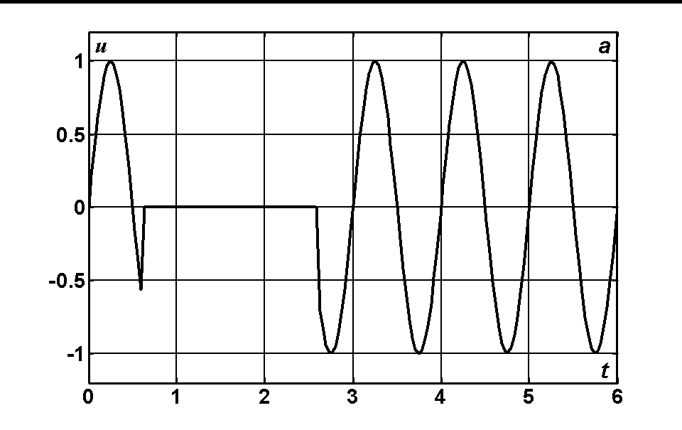
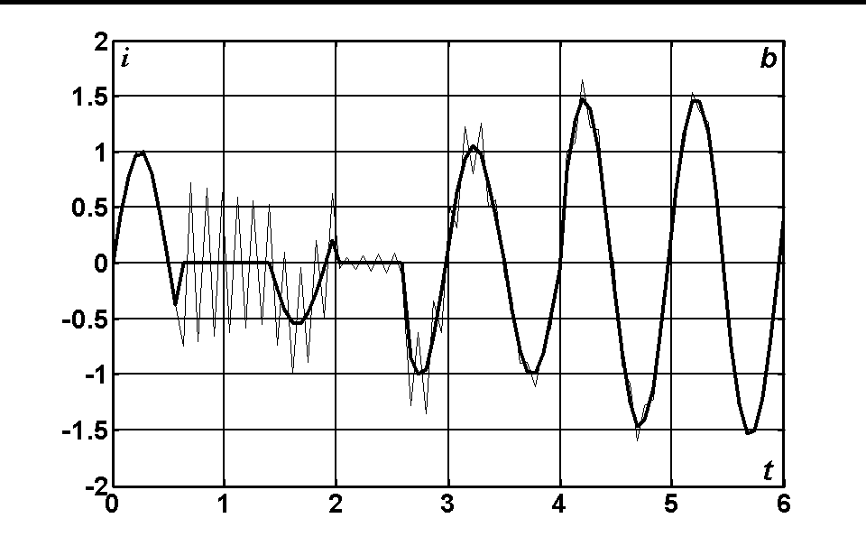
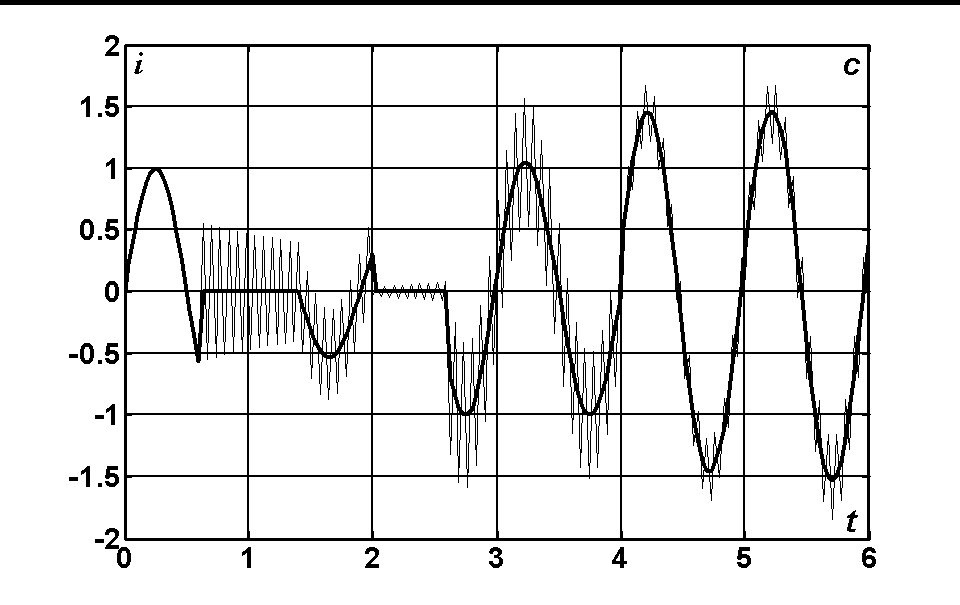
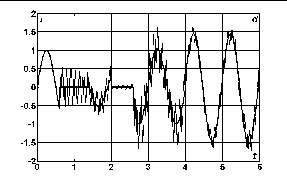
Fig. 2.1. The time dependence of the voltage at the input of the line (a) and of the current when N = 10 (b); N = 20 (c); N = 40 (d).

The given figures demonstrate that the FDTD method on discontinuous solutions leads to the appearance of large oscillations that do not decrease with decreasing of the grid step. But there is no reason to be surprised since as early as 1959 it was proved by Godunov [5] that among the linear finite difference schemes with second order of accuracy for the equation

there is no one satisfying the condition of monotony, i.e. no one that does not lead to appearance of the oscillations when computing the discontinuous solutions.

Thus, the FDTD method, in spite of the fact that it is of second order of accuracy, can be restrictedly applied to the telegraph equations as it does not permit the modeling of such regimes as short-circuit and idling.

Conclusion

1. The finite difference schemes obtained by means of FDTD method and by means of Godunov’s scheme are considered.

2. It is demonstrated that the FDTD method can not be applied to simulate the short circuit and idling processes.

References

Kane Yee. Numerical solution of initial boundary value problems involving Maxwell's equations in isotropic media. Antennas and Propagation, IEEE Transactions on. Vol. 14. p. 302–307.
Taflove A. and Brodwin M.E. Numerical solution of steady-state electromagnetic scattering problems using the time-dependent Maxwell's equations. Microwave Theory and Techniques, IEEE Transactions on. Vol. 23. p. 623–630.
Taflove A. and Brodwin M.E. Computation of the electromagnetic fields and induced temperatures within a model of the microwave-irradiated human eye. Microwave Theory and Techniques, IEEE Transactions on. Vol. 23. p. 888–896.
Patsiuk V. Mathematical methods for electrical circuits and fields. – Chisinau: CEP USM, 2009. – 442 p.
Godunov S.K. Finite difference method for discontinuous solutions of hydrodynamics problems. Math. Coll. 1959, vol. 47(89), ser. 3, p. 271 – 306 (in Russian).

V. Patsiuk. Doctor of phys.-math. sc., Associate Professor at Moldova State University, Research Fellow at the Institute of Power Engineering ASM. Scientific interests: mathematical physics, numerical analysis, mechanics and theoretical electrotechnics. Author of about 90 scientific works including 10 monographs.

G. Ribacova. Doctor of phys.-math. sc., Associate Professor at Moldova State University, Research Fellow at the Institute of Power Engineering ASM.. Scientific interests: mathematical physics, numerical analysis, mechanics of deformable solids. Author of about 40 scientific works.

Blog

Curacy of numerical solutions received by Finite Difference Time Domain (fdtd) method and Godunov's method at the solution of the cable equations is carried out

Содержание